B. Morgan – Page 2

Differential Photometry of Delta Scuti Variable Star “YZ Boo”

By B. Morgan | April 9, 2020

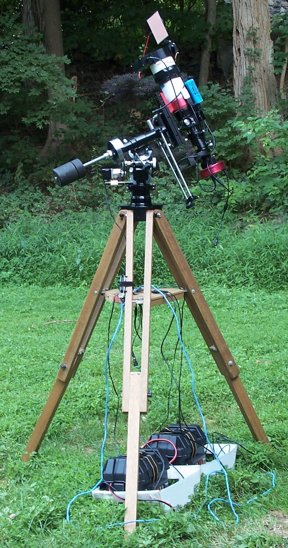
I am always interested in finding things to do with my kit when the Moon interferes with normal wideband astrophotography. Last night the Moon was full so I turned my attention to a variable star in Bootes designated “YZ Boo”. It is a 10th magnitude star that fluctuates in brightness from approximately 10.3 to 10.8 with a period of 2.5 hours. It is one of my favorites:

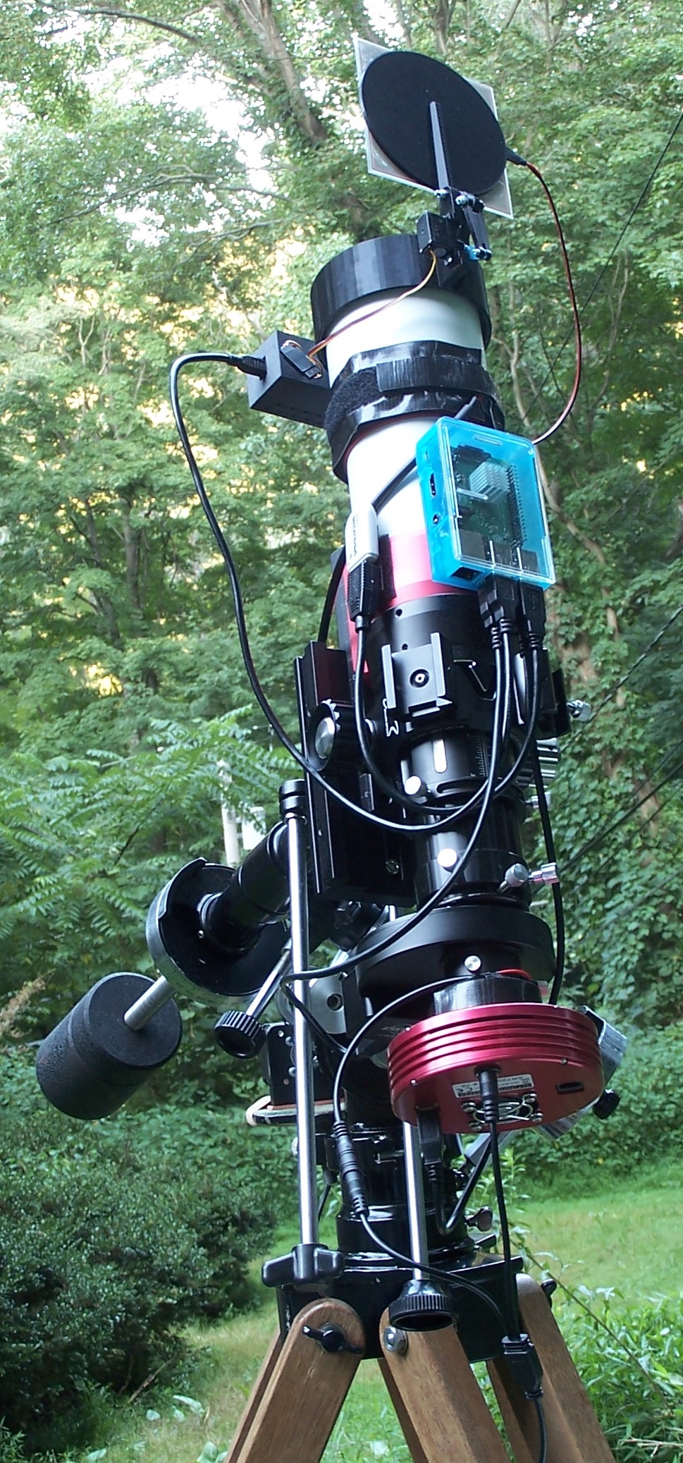
Seeing conditions rapidly declined, not only due to the Moon, but also a storm front that moved swiftly towards me. When I began imaging there was a feeling of dampness in the air but nothing severe. By the end of the 2 hour session my equipment was wet with dew (thankfully my DIY dew heater bands around the objective lens and one around the nose of the CCD prevented disaster.)

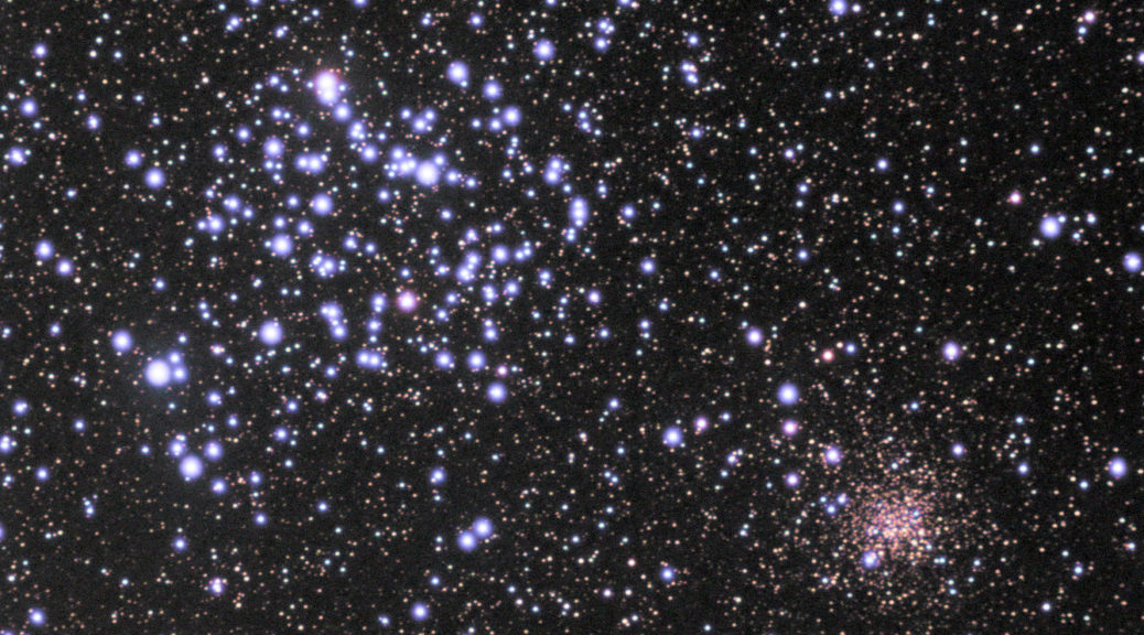
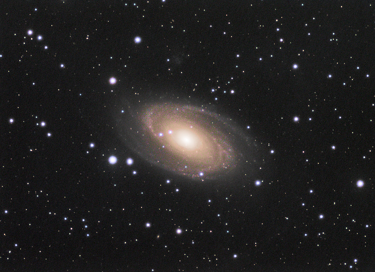
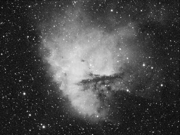
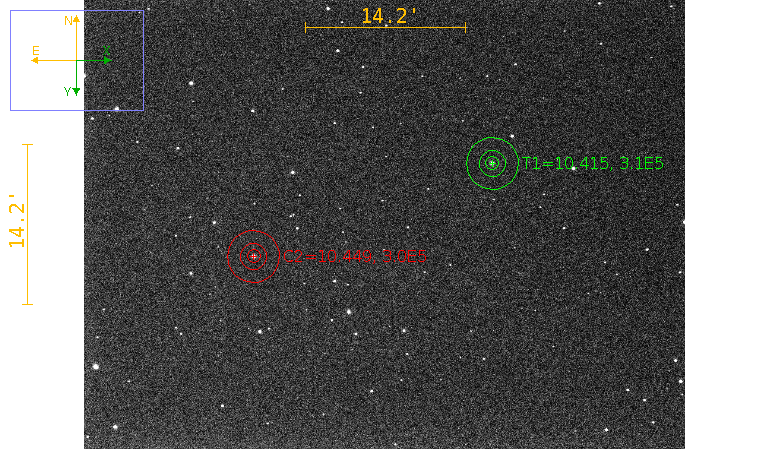
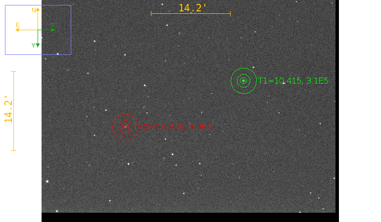
You can see how a blanket of damp air descended on me from the first frame:

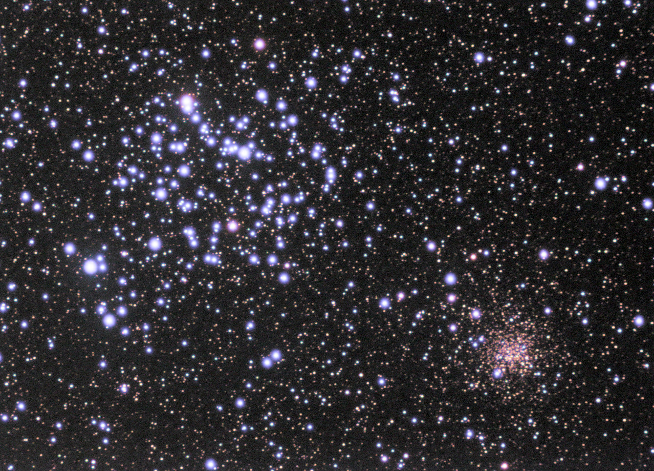
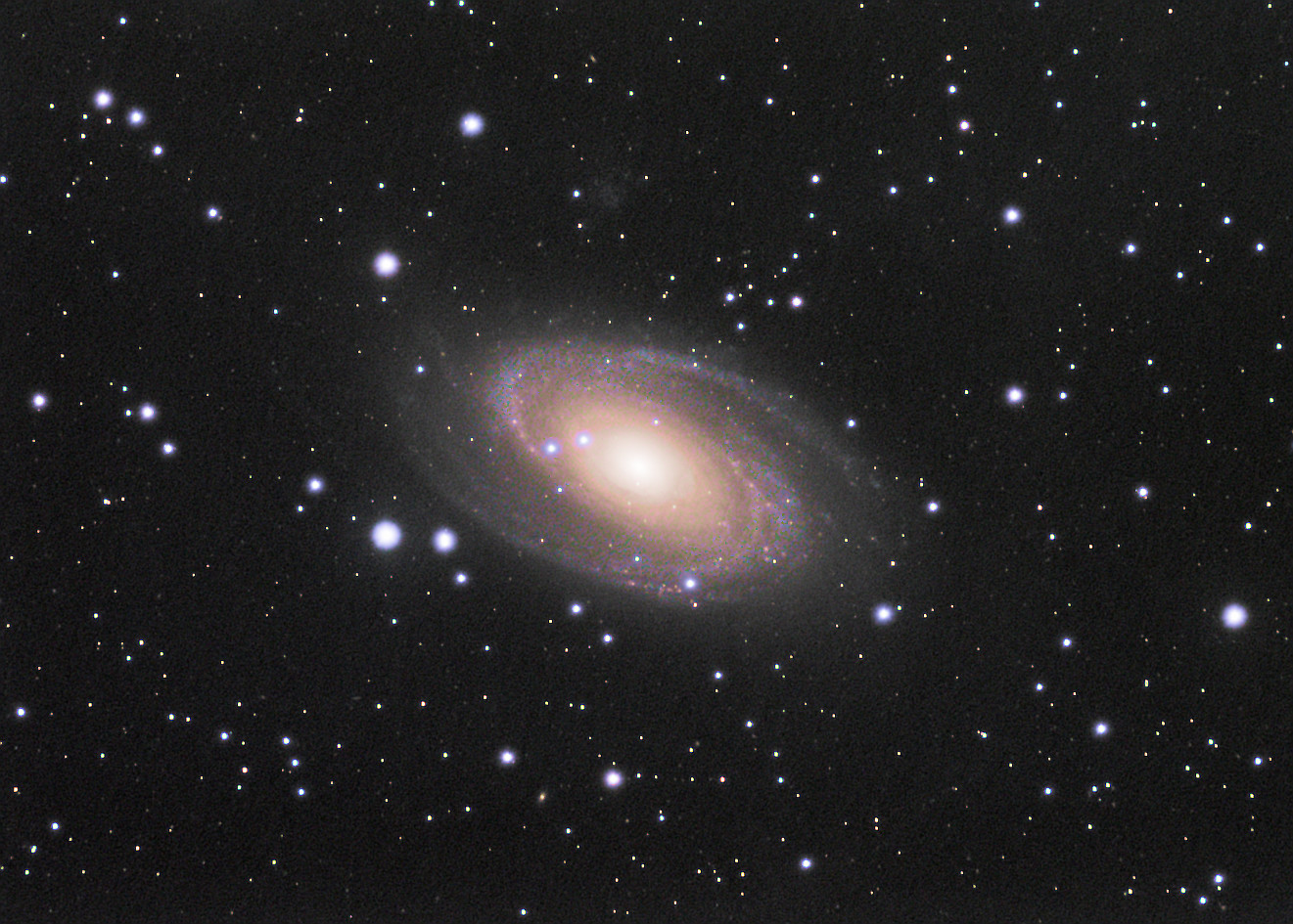
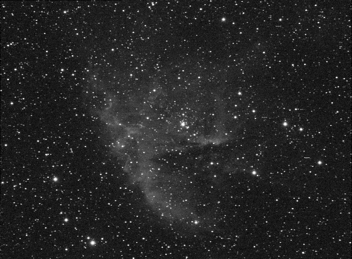
to the last frame:

I had to cut the session short after 2 hours when thick clouds arrived.

I decided on a 50s exposure that placed the star near the midpoint of the camera’s 16-bit range, around 30,000 ADU. Thankfully the field included a few constant-brightness stars, one of which I used for comparison.

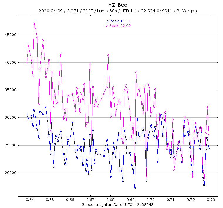
Here is a plot of the peak pixel value over time. Look primarily at the pink plot. It is the constant-brightness comparison star. You can see how the peak steadily declined as the damp air increasingly blocked starlight:

The next plot requires some explanation. If you look back at the First and Last Frames you can see that I placed an “aperture” on the variable star (T1) and the comparison star (C2). The central bulls-eye is designed to surround the star so that starlight can be integrated over its area. Then there are two annulus rings: the inner annulus and the outer annulus. The outer annulus is used to sample the sky background. The inner annulus is simply a buffer between the aperture and the outer annulus.

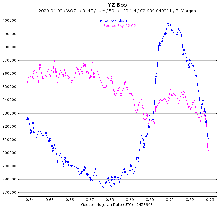
This plot is the difference between the aperture and the outer annulus. Notice how we are getting closer to the final light curve:

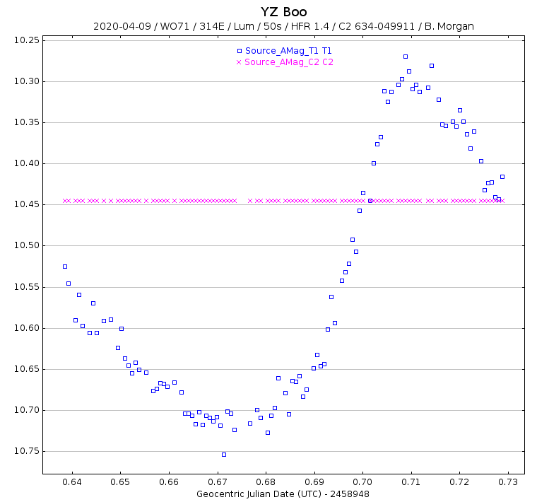
There is one step left. We need to calculate the difference between the blue plot (the variable star) and the pink plot (the comparison star). This yields the final light curve:

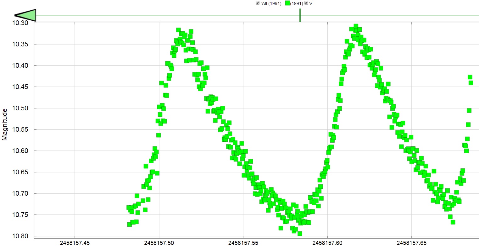
For comparison here is the light curve of YZ Boo contributed by members of the American Association of Variable Star Observers (AAVSO). These people have some serious equipment including CCD cameras having a Full Well Depth of 100,000 electrons:

I used a free package called AstroImageJ for calibration, alignment and photometry. It is easy to use once you run through it a couple times. Also, AAVSO’s Variable Star Index (VSX) is available online to members and non-members alike. With it you can search a vast database of variable stars that meet your criteria. You don’t necessarily need costly photometric filters to have fun. I used a standard luminance filter but I do have Astrodon Photometric “V” and “B” filters on another filter wheel.

Star Clusters: M35 + NGC 2158

By B. Morgan | March 11, 2020

Fifty years ago when I became interested in Astronomy my first telescope was a refractor designed for lunar and planetary work. That first year Mars came closest to Earth. I was amazed to see land features and polar ice caps. Jupiter’s cloud system and four of its brightest moons were easily seen and Saturn was gorgeous.

When I turned my telescope to galaxies I was disappointed. People call them “faint fuzzies” for a reason: they are faint and they do look like fuzzy stars. I wanted to see what professional astronomers see with their large telescopes. I resigned myself to reality and gave up on them with the equipment I had.

One favorite target, besides the planets and the Moon, were star clusters. I dabbled in astrophotography using photographic emulsions like Kodak Tri-X and Spectroscopic 103a-E. Some of my best photographs as a teenager were star clusters.

These days star clusters don’t get the respect they deserve. People do like the famous M13 Hercules Globular Cluster but that is the exception rather than the rule. I decided to try my hand at star clusters again with my new equipment. The great thing about star clusters is that they are bright compared to galaxies and nebulae, and because of that you can tolerate the Moon within reason.

Successfully imaging a star cluster requires a new set of rules. Your audience’s attention is focused on the stars themselves and because of that you want to avoid overexposing them as much as possible. When they reach overexposure they saturate the camera’s pixels and spill over to surrounding pixels. Eventually the surrounding pixels reach saturation and then spill over into more pixels. To me a saturated star looks unpleasantly large and unappealing. Sometimes, though, you can’t avoid some amount of saturation especially when there are many fainter stars that you also want to capture.

The technique I used is described here at my sister site: https://snrcalc.now.sh/help/open-star-clusters

Open Star Clusters: M35 (bright blue stars) and NGC 2158 (faint red stars)

Telescope: William Optics ZenithStar 71mm f/5.9
Camera: Atik 314E CCD (Read Noise 5.3e-, Full Well Depth 13400e-)
Filters: Optolong LRGB
Mount: Unitron Model 152
Tracking: Self-designed R.A. stepper motor with PPEC on Raspberry Pi 3B
Image Acquisition: Astroberry INDI/Ekos on Raspberry Pi 3B+
Remote Guiding Assistance and Polar Alignment: SharpCap 3.1
Image Processing: AstroPixelProcessor (APP) version 1.076

Over three sessions:
L: 540x15s bin1, 2.25 hours
R: 300×14.3s bin2, 1.2 hours
G: 300×8.4s bin2, 0.7 hours
B: 300×13.0s bin2, 1.1 hours
Total Integration time: 5.23 hours

The odd-looking exposure times are due to how I color balance my RGB filters. In many cases this leads to an image that requires no further color adjustments but in this case the image was a tad bit green, so I used APP’s color calibration tool. Why this was necessary was a challenge to solve but now I understand. I designed a spreadsheet to solve the problem. Going forward I will use it as part of my image capture program.

What a difference two years makes

By B. Morgan | February 29, 2020

I am writing to affirm that progress is inevitable but only with heaps of patience and experimentation.

Two years ago I had the same telescope as today. So what’s the difference? The camera, but not what you think. It was how I was using it.

The top image, the one in color, was taken with the Atik 314E CCD, and the bottom image with the Altair 290M CMOS camera.

Don’t get me wrong. I’m not making a pitch for CCD over CMOS. I am saying that the exposure you choose makes all the difference in the world.

The bottom image used the subframe exposure of 4.7 seconds. Total integration time was 60 minutes. It may not be clear in this small image but it suffered from a severe case of “raining noise”. This was a common ailment of my early images. Without going into a lengthy explanation the cure was to increase the exposure.

The question is always “How far do I increase the exposure?” You can always experiment. A good test is to keep the total integration time the same, in my case 60 minutes, but you can choose 30 minutes if you want to test a greater range of exposures in one evening.

For the Altair 290M and my Bortle 5 skies it turns out that 30 seconds is optimal. You can increase it farther but image quality, signal-to-noise (SNR), won’t improve that much. You can decrease the exposure but then you will see a dramatic drop-off in SNR. If you decrease exposure too far then “raining noise” will rear its ugly head.

Of course the “optimal” exposure is completely dependent on your skies, your telescope, and camera.

The top image was taken with the Atik 314E using a 90-second exposure over 11.6 hours and LRGB filters. The signal-to-noise ratio is high due to the long integration time so comparing it to the bottom image is not entirely fair. The important point is that “raining noise” was never a problem. I chose a 90-second exposure because a CCD has higher Read Noise than a CMOS camera. I could have gone down to 60 seconds but below that the image would have suffered.

M81 Bode’s Galaxy in 11.6 hours

By B. Morgan | February 26, 2020

Over five sessions:
L: 250x90s bin1, 6.25 hours, SNR 17.78
R: 90×85.8s bin2, 2.13 hours, SNR 10.74
G: 90×50.2s bin2, 1.26 hours, SNR 10.66
B: 90×77.8s bin2, 1.95 hours, SNR 10.63
Total Integration time: 11.59 hours
Total target SNR: 25.65

A quick survey of AstroBin reveals a startling variation of colors from members’ images of M81. One would think that there should be consensus. Top Picks did converge on a color scheme where the core is yellow and the arms are blue. I was keen on duplicating that result with little post-processing since I meticulously white balance my RGB filters. (This explains the strange looking exposure times that I use.)

I chose this Top Pick image at AstroBin as an accurate depiction of the galaxy’s color https://www.astrobin.com/385501/0/ . Notice he invested 30 hours to capture it. My method reduced the time to about 12 hours but I forfeited detail to achieve it.

Thankfully my equipment worked flawlessly but I did have to cope with a user error (me) on the last night from which I was able to recover.

Problems began during post-processing. The color balance was off. The galaxy was predominantly yellow with just a hint of blue in the outer arms. Here is that initial image:

The initial image was too yellow, not enough blue.

It took a day to solve but first let me explain that unlike a lot of astrophotographers I do not like to rely on software to perform color balancing. I prefer to get it right at the telescope.

A key component of my color balancing strategy is to white balance my filters against a Sun-like star. What I failed to realize is that there needs to be another component that accounts for atmospheric extinction. Atmospheric Extinction is an estimate of the amount of atmosphere between you and the galaxy. It is a function of the galaxy’s altitude above the horizon. The brightness diminishes the closer to the horizon, and grows as it reaches overhead.

I’ve known of atmospheric extinction and its effects for quite some time. I’ve chosen to mitigate its effects by selecting the red filter first, followed by green then blue. This is for objects east of the meridian. This strategy worked well up until this galaxy M81.

The essential difference between a galaxy like M81, Bode’s Galaxy, and M31, the Andromeda Galaxy, is that M31 faces east and M81 is circumpolar. Circumpolar means that it never sets since it is so close to Polaris. This also means that M81 never gets very high in the sky. It reaches 62 degrees above the horizon whereas M31 almost reaches 90 degrees. M31 becomes much brighter in the telescope when it is close to overhead. M81 never reaches those heights. The end result is that M81’s blue filtered images are less bright than M31’s.

I performed a mathematical analysis and discovered that M81’s blue stack of images is less bright than its red stack. This explains why the initial print of M81 is so weak in blue.

One solution is to go back to the telescope and capture more blue images. A second solution is to delete some of the 90 red images but keep all 90 blues. A third solution is to leave the images alone and to use the controls in AstroPixelProcesssor (APP) to attenuate the red stack. I chose to do the latter.

To get the color balance right I needed to attenuate the red stack by 17% and the green stack by 10% while keeping the blue stack at 100%. Here is the final processed image:

I have since developed a spreadsheet to assist me in capturing the proper number of images per filter. I’ll use that going forward.

Tadpole Nebula (IC 410)

By B. Morgan | December 25, 2019

These past few months I developed an interest in narrowband imaging mostly out of necessity due to the Moon. It turns out to be more challenging than I thought. One of my heroines in the field is Sara Wager. I recommend her website for anyone seeking to discover the secrets to good narrowband imaging. I’d like to share some with you:

Stretch your stacks before combining. You may notice that imaging in Hydrogen Alpha (Ha) is easy due to the strength of the signal. Oxygen III (OIII), on the other hand, is relatively weak. To prevent Ha domination you should stretch your OIII stack before combining them into a single RGB image. By how much? It all depends, so experimentation is the key.

Figure A shows the relative strength of Ha (left) compared to OIII (right). These images were equally “stretched” using Astro Pixel Processor (APP) software. If I were to combine these two into a color image then you would mostly see red with only a few light red regions. You could make the argument that this is how it exists in nature, and you would be correct, but we are striving to show chemical composition, not necessarily quantity:

Figure B shows Ha stretched less and OIII stretched more. How much you stretch is a matter of taste. I wanted to come close to Sara Wager’s image.

Figure C is the final color image obtained by assigning 85% of Ha to Red, 65% of OIII to Blue, and the remaining amount to Green. This creates a pleasing range of colors:

How to interpret the colors:

Blue/Cyan on the left side of the image is predominantly oxygen.
Scarlet/Orange on the right is almost pure hydrogen.
Beige in the center of the nebula is a mix of hydrogen and oxygen.
The “tadpoles” have hydrogen tails and oxygen/hydrogen heads.

Here are some other best practices that I learned from Sara Wager:

When combining stacks to create a color image try not to assign a stack to a single channel. For example the “HOO” palette says to assign Ha to Red but if you do that it will render as brilliant red. A more appealing color is scarlet to orange. You can accomplish this by assigning, say, 85% to red and 15% to green.

You need star size reduction software. There are lots of hot blue stars in the sky that strongly emit at the wavelength of OIII. You may have noticed that stars saturate easily in your OIII frames and therefore are fatter than stars in your Ha and SII frames. As a consequence your image will suffer from what I call “oxygen halo”. Also fat stars detract from your subject. Photoshop and PixInsight have tools for reducing star size but they are expensive. StarTools also has a tool. Two years ago I purchased StarTools for $50 for a single license that never expires. It is still available for sale at the same price.

Technical Details:

William Optics 71mm f/5.9
Atik 314E CCD (slightly undersampled at bin1 so bin2 is worse)
Orion 6nm Ha and OIII narrowband filters
Unitron Model 142 German Equatorial Mount.
Tracking: Own design Permanent Periodic Error Correction (PPEC) using stepper motor and Raspberry Pi Model 3B.
Flat-fielder: Own design “The Flatinator”

Image Capture:
Astroberry/INDI/Ekos on Raspberry Pi Model 3B+.
SharpCap for guiding assistance, polar alignment, and PEC learning.
Ha: 18x600s (bin2 to boost signal to keep exposure time to 10 minutes.)
OIII: 23x600s (bin2 also)
Total integration time: 7 hours.

Image Processing:
1. Astro Pixel Processor (APP) for image calibration, integration, stretch, and composition. 2x drizzle to repair square stars and restore image dimensions to bin1.
2. StarTools for star size reduction and additional image processing.

HOO palette:
Ha: Red 85%, Green 15%
OIII: Green 35%, Blue 65% (stretched before combine as shown in Figure B)

High Dynamic Range (HDR) Photography using Photomatix

By B. Morgan | December 4, 2019

While I wait for the weather to improve for astrophotography I discovered High Dynamic Range (HDR) photography through a friend in Great Britain. HDR is commonly used by real estate agents to capture beautiful sun-drenched living spaces. Astrophotographers have used HDR to capture stunning images of the Crescent Moon bathed in Earthshine and images of Total Solar Eclipses. There might be other applications that I want to explore.

Many years ago I was heavily engaged in conventional photography of landscapes and portraiture. This was at a time before digital photography. Portraits were the easiest to capture since they were obtained in a controlled environment of a studio. Shadows that would normally render in black could be filled with flash or flood lights. Highlights that would normally appear washed out on film could be softened with light diffusers.

By far the most difficult was landscape photography. There you didn’t have the option of using flash, flood lights, or light diffusers. You relied more heavily on darkroom techniques. Things changed with the advent of digital photography.

Photomatix is a software product from HDRsoft Ltd, a UK company. They have several versions, some that integrate well with Photoshop, others that are standalone applications. I chose the standalone version for Linux since I find myself increasingly turning away from Windows in favor of Linux. The trial version never expires and is full-featured but they do draw the Photomatix watermark on your final image. The cost of a license is reasonable at $49. For this test I am using the trial version. The software is very easy to use plus there are many videos available on YouTube to learn how to use it to its fullest extent.

The difficult part is capturing the images. Instead of me yammering on attempting to explain what to do, allow me to present the seven photos that I input into Photomatix:

The essential parts of the scene are the sky, the snow, the car, and the snow on the limbs of the trees. The sky and the snow on the ground are the brightest parts. The car and tree limbs are the darkest. The objective is to capture detail in all of them. Notice that there is no single exposure that satisfies us. Perhaps the closest is “exp 60th” but notice how the sky is completely blown out. This scene is a perfect candidate for HDR using Photomatix.

Notice that my exposures range from 1/1000s to 1/15s. I chose 1/1000s because it showed the best detail in the sky and the snow on the ground. I chose 1/15s because it showed the best detail in the car and the tree limbs. Once I determined those endpoints then I proceeded to capture images in full-stop increments: 1/1000s, 1/500s, 1/250s, 1/125s, 1/60s, 1/30s, 1/15s. It is important to keep the same f/stop. In my case it was f/7.

My camera is rather old so it does not have auto-bracket mode. No worries, I used manual mode instead. My camera has an integrated spot meter. Wherever I point the camera it will read out if it is under-exposed or over-exposed. The meter readout is around the center of the view.

The steps are:

Choose an f/stop.
Adjust the zoom to frame the scene as you like.
Point the camera at the brightest part of the scene, in my case the sky and ground snow.
Adjust the exposure setting so that the meter reads zero (neither under-exposed nor over-exposed). Make a mental note, in my case 1/1000s.
Point the camera at the darkest part of the scene, in my case the car and tree limbs.
Adjust the exposure so that the meter reads zero, in my case 1/15s.
Attach the camera to a tripod.
Double-check the framing.
Click the button to capture the frame. (This should be at our current setting of 1/15s.)
Adjust the exposure one full-stop, in my case 1/30s.
Click the button to capture the frame.
Repeat these steps until you capture the last frame at the terminal exposure, in my case 1/1000s.

That’s it! Download the images to your computer and process in Photomatix. I’ll leave that activity for you to figure out. There are plenty of video resources for that. Good luck!

What makes the PacMan Nebula light up?

By B. Morgan | October 7, 2019

A former co-worker who has an interest in astronomy prompted me to answer the title question: “What makes it light up?”

To understand what is happening look at a neon sign. It is made up of a tube of neon gas atoms. On both ends of the tube a very, very high electric voltage is applied. The electric energy temporarily strips a neon atom of one of its electrons. A fraction of a second later that electron rejoins the atom and when it does a photon of light is emitted. The wavelength of that light is very “narrow”.

Notice how I used the term “narrowband” in the previous post. What this means is that I use a filter that passes only a narrow band of light. Different atoms emit different wavelengths of light. Hydrogen is different from sulfur which is different from oxygen. By using different filters I can tell which elements make up a cloud of gas in outer space.

The last question to answer is where does the “very, very high electric voltage” come from in outer space? The answer is that it doesn’t have to be an electric voltage, just something that is highly energetic. If you look at the center of the PacMan nebula you will see a bright star and several stars around it. That cluster of stars emits a lot of energy which causes the gaseous nebula to light up somewhat like a neon sign!

The PacMan Nebula is known as an “emission nebula” not to be confused with a “reflection nebula”.

PacMan Bi-Color Ha-SII-SII with only 2 hours of data

By B. Morgan | October 7, 2019

Having recently broken the sound barrier with improvements to my Raspberry Pi’s tracking software, I am now able to take unguided 8-minute exposures.

I set out to capture the PacMan nebula (NGC 281) in narrowband in order to do a full Hubble Palette but the weather turned ugly so I was only able to capture one hour in Hydrogen-alpha (Ha) and one hour in Sulfur-II (SII). According to forecasts the weather won’t improve for at least a week.

Here is what I have. I don’t think it is too bad considering that top-tier images in narrowband have at least 10-20 hours of data compared to my 2 hours. Another negative going against me is that my f/5.9 refractor is a bit too slow for this type of work, and my Atik 314E is not at all sensitive to the red part of the light spectrum. This is why I image in bin2 mode. If you zoom in you can see that my stars are square. These deficiencies can be solved in a variety of ways but for now this is what I have.

How to interpret the colors? By in large this is a hydrogen gas cloud with hints of sulfur (and oxygen that I haven’t captured yet) but it is predominantly hydrogen. The dark red areas are almost 100% hydrogen, the lighter red to nearly gray is sulfur plus hydrogen.

Ha is assigned to the red channel, SII is split 50% to green, 50% to blue, and then SII is boosted 2x. The 2x boosting allows SII to play a prominent role but boosting also means doubling the noise. In the future I will plan on capturing two to four times more SII frames.

For perspective here is the Ha stack:

and here is the SII stack:

when those two are combined you get the color image above.

If you zoom in on the SII image you may notice that the stars are elongated whereas the stars in the Ha image are nearly perfect. The reason is that the atmosphere was particularly turbulent during the hour I captured the SII frames. The ambient temperature dropped at a high rate of 2 degrees Celsius per hour. Thank you to Dr. William G. Unruh, Professor of Physics & Astronomy at University of British Columbia for pointing that out.

Andromeda Galaxy (M31) The Saga Continues: Siril + APP.

By B. Morgan | September 27, 2019

This is only half of the galaxy. The core is at the lower-left and the arms stretch outwards to the upper-right. To visualize how large it really is, imagine the Full Moon. My camera can just about fit the Full Moon in its frame!

UPDATE: I want to thank Mabula Haverkamp, author of Astro Pixel Processor (APP). Beginning with version 1.075 APP successfully processes this image. The original story was written using version 1.074. As you read you can see that I had to fallback to using Siril which is no longer the case. The image shown above is part of the original story which used Siril for star alignment and stacking. While it was successful the alignment was not perfect. If interested you can see the high-quality APP image here: https://u235.herokuapp.com/#lrgb-exposure and scroll two-thirds of the way down.

Original story:

The night of this shot I was blessed with excellent seeing conditions, a rarity in this part of the country. The atmosphere was calm. Stars were stable. On most nights however the atmosphere is quite turbulent, causing starlight to rapidly twist and turn.

Sounds idyllic, right? Well, yes and no. On the one hand I can capture some very fine detail which normally would be lost to poor seeing conditions. On the other hand however the small size of the stars on the camera’s sensor can lead to a condition called “under-sampling”.

Ideally you want the average brightness star to cover a 3×3 area of pixels. With average to poor seeing conditions this is no problem but with excellent seeing conditions the star may only cover a 2×2 area.

After capturing the image at the telescope I began processing with Astro Pixel Processor (APP). Almost immediately it complained that it could not find enough stars in the color frames! I was shocked but not surprised.

When I purchased this CCD camera I knew that it had a tendency to under-sample (see notes at the end of the article.) This condition is exacerbated when capturing color frames using bin2 mode. Bin2 can dramatically reduce the exposure time of color frames but there is a downside. It cuts image resolution in half because it reduces each 2×2 matrix of pixels to one pixel.

This isn’t as terrible as it sounds. I think it was Trevor Jones at AstroBackyard who made the analogy of a child and his coloring book. The child provides the crayons and the publisher provides the detail in the form of the outline. If the child draws a little outside the outline the picture still looks good. If he gets sloppy it gets worse but is still acceptable especially if seen from a distance. This is the analogy that Trevor made with binning: bin2 is like the child drawing a little outside the outline, and bin3 is sloppy but acceptable. Remember that the outline is the job of the luminance filter running at bin1 and since the sensor sees three times more photons than with a color filter the exposure time is short.

So Astro Pixel Processor did not like my bin2 color frames. I checked the log file. Initially it said it found 100 stars but ultimately decided that only 4 of them qualified as real stars. Apparently the software looks at the star’s profile. Since there were so few pixels it failed.

I contacted my friend David Richards in the UK. He suggested I try Siril. I dedicated several hours and took a crash course from the online tutorial guide. Soon thereafter I had a reasonable looking final image. Thanks to Dave he helped me with some of the finer points of using Siril and now I have this wonderful image that you see here.

The subtitle of this blog post is “The Saga Continues”. It never ends but with regards to this image there is much more to say. I’ll leave that to a later post.

Technical Details:

William Optics 71mm f/5.9
Atik 314E CCD
Optolong LRGB filters

Luminance: 38x120s bin1
Red: 18x90s bin2
Green: 10x90s bin2
Blue: 17x90s bin2

Bias: 100 each for bin1 and bin2
Darks: 50 each for 120s bin1 and 90s bin2
Flats: 50 each filter

Total Integration Time: 2.4 hours

Siril for calibration, stacking, and color balance.
APP for histogram stretch and sharpening.

Note: Before purchasing an astronomy camera, no matter if it is CCD or CMOS, you should make sure that you match the camera to your telescope. Astronomy Tools has an excellent resource called the CCD Suitability Calculator. Scroll to the bottom of the page. There are two boxes I want you to fill in. Focal Length: 418. CCD Pixel Size: 4.65. Notice the warning: “this combination leads to slight under-sampling.” Now change CCD Binning from 1×1 to 2×2. Notice it goes off into the red. Ideally for 1×1 binning you want the indicator to be at the lower end of the green region and for 2×2 binning at the higher end of green. For my telescope that would be a camera with a pixel size of about 2 microns.

My Gear

By B. Morgan | August 12, 2019

Here are recent photos of my telescope as I was setting up to image the Andromeda Galaxy Mosaic. Noteworthy items include:

Astroberry/KStars/Ekos/INDI using RasPi Model 3B+
Unitron Model 152 German Equatorial Mount (50 years old and running great)
William Optics ZenithStar 71mm f/5.9 (20th Anniversary Edition)
Atik 314E CCD (used, approximately 10 years old)
ZWO 5-filter Electronic Filter Wheel (EFW), Optolong LRGB filters, and Orion dark filter
Altair 290M CMOS camera & 200mm finder/guider scope for polar alignment (not pictured)
Flatinator flat-fielder and dust cover (my own invention)
Permanent Periodic Error Correction (PPEC) using RasPi Model 3B and Stepper Motor (my own invention)
OMC Steppers-Online Motor with 26.85:1 Gearbox
Dew heater strips on objective and sensor window (DIY from plans by “DewBuster”)
Two Interstate DCM0035 12VDC 35Ah Deep-Cycle Batteries
Two West Mountain Radio U1 Battery Boxes with fused distribution panels
Various PowerPole connectors and USB cables
One DROK 12VDC Buck/Boost Converter for regulating power to the camera
Two Adafruit UBEC 12VDC-to-5VDC regulators for powering the RasPi’s
One Adafruit Stepper Motor HAT for RasPi