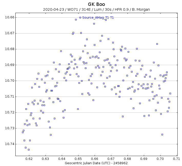
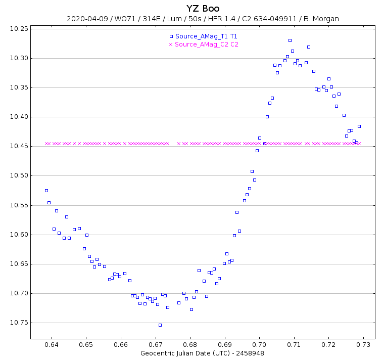
The data that I presented in Part 1 was from a single session on April 23, 2020 however I also captured data on April 19, 2020 but unfortunately it suffered from poor tracking. Nevertheless it is still useful for demonstration purposes.

Before I present the second data set allow me to briefly describe the software I use:

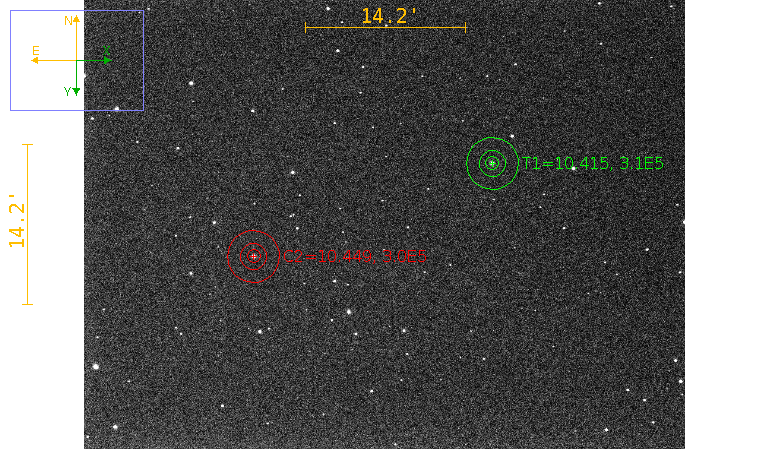
AstroImageJ, henceforth referred to as AIJ, enables me to calibrate and align frames (and stack if I so wish.) More importantly I can perform Differential Photometry. The one drawback from my perspective is that it is designed for Exoplanet research and therefore expects me to capture the entire light curve in a single session, however my requirements differ in that the period of most variable stars far exceeds that.

VStar, a Java application from AAVSO, enables me to view my data over multiple sessions. Using it I can switch between two modes: Light Curve and Phase Plot. Light Curve mode is similar to AIJ in which the horizontal axis is in units of time. Phase Plot mode requires me to know something about the period of the light curve. It takes that information and then “folds” my observations onto a phase scale from -100% to +100%.

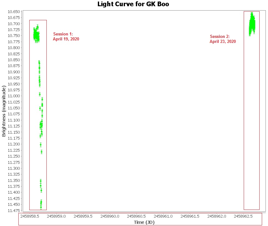
In the following screenshot I used VStar to plot the two sessions in Light Curve mode. Notice how the data is compressed horizontally. This is due to the fact that four days separated the first and second session:

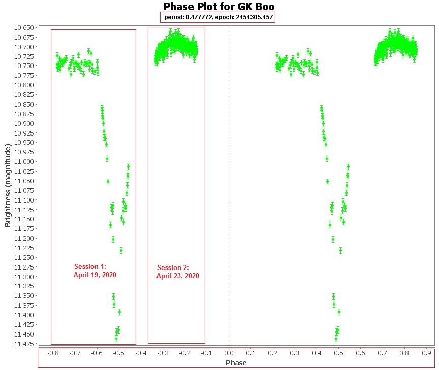
This next screenshot uses VStar’s Phase Plot mode. I entered GK Boo’s period obtained from the AAVSO database:

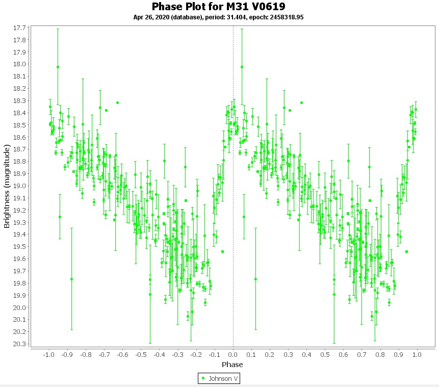
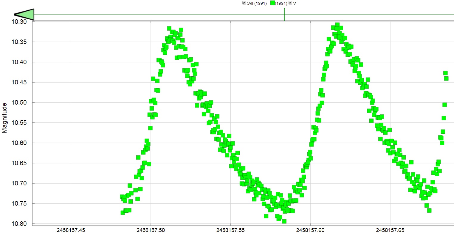
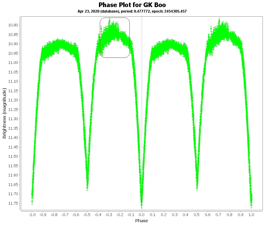
Compare the Phase Plot of my data to that of all data from members of AAVSO, seen below. (Please ignore the red box drawn atop one of the peaks. This image is being shared from an earlier post.) Notice the similarity:

Phase Plot mode is essential since some variable stars take a year or more to capture and can span dozens of sessions.

On October 6, 1923 renowned astronomer Edwin Hubble discovered a pulsating star in the Andromeda Galaxy which quickly led to the revolutionary discovery that M31 is a galaxy unto itself 2.5 million light-years away, and not a gaseous cloud of stars within our own Milky Way.

I dipped into my archive of astro images to see if I might have captured that same variable star. I did! In the attached image I’ve overlaid a small region of a 6-panel mosaic I made last year, atop Hubble’s photographic plate he captured with the 100-inch telescope at Mount Wilson Observatory. You can see that the pattern of stars matches nicely. At the point of the arrow that I marked “VAR!” you will see an equilateral triangle of faint stars. You can see that it matches up with Hubble’s. That one star at the vertex of the triangle is the famous variable star.

My image is a stack of 21x 90-second luminance frames captured with a cooled Atik 314E CCD and William Optics 71mm f/5.9 refractor under Bortle 5 skies. Total integration time is 31.5 minutes. I know nothing of the period of this variable star. Being a Cepheid type variable star its period is most likely one or more days in length, so integrating for 31.5 minutes is not a problem. The bigger question is, am I seeing it at minimum light or maximum light? I almost don’t want to know. I want to feel the same sense of discovery as Hubble did.

EDIT: I suspect that this variable star is likely to have a long period perhaps months long. I suspect this because of the “period-luminosity relationship” which says that highly luminous Cepheids have long periods. This star must be highly luminous if I can see it as a point source from such a great distance. If it was less luminous it would be lost in the glow of the galactic arms.

I will make this one of my top priority projects this Fall: measure the period of the variable star, and then calculate its distance using Leavitt’s Law.

https://apod.nasa.gov/apod/ap200426.html
https://apod.nasa.gov/apod/ap950701.html
https://astrotuna.com/andromeda-galaxy-mosaic-as-of-2019-08-12/

AAVSO’s official designation is M31 V0619. They report that its magnitude fluctuates between 18.5 and 19.8V. That is faint. I’ve known that my scope/cam can see down to 18th magnitude at my Bortle 5 site but can it see down to 19th magnitude? What makes things worse is that the star is embedded in the glow of a spiral arm which further reduces the signal-to-noise ratio. There is only one way to tell. Do it!

I was curious as to what phase the star was in when I captured my image. According to the AAVSO’s Ephemeris it reached maximum light on July 31, 2019 07:08 UTC. My image was captured August 3, 2019 02:00 UTC. So, three days after maximum light. That pretty much puts it at magnitude 18.5.

Here is the Phase Plot contributed by ten AAVSO members between 2010 and 2019. Ignore the outliers.

Today’s NASA Astronomy Picture of the Day (APOD) is a celebration of the 100th anniversary of astronomy’s Great Debate held at New York’s Museum of Natural History between Harlow Shapley and Heber Curtis. Shapley argued that the Milky Way was the size of the known universe and that the Andromeda Nebula (M31) was part of it just like the Orion Nebula (M42). The debate ended with no decision either way. In fact Shapley’s model was accepted for years until Edwin Hubble and Henrietta Leavitt revolutionized the scale of the universe and proved that the Andromeda Nebula was in fact its own independent galaxy. 100 years ago today!

https://apod.nasa.gov/apod/ap200426.html
https://en.wikipedia.org/wiki/Great_Debate_(astronomy)
https://en.wikipedia.org/wiki/Edwin_Hubble
https://en.wikipedia.org/wiki/Henrietta_Swan_Leavitt
https://en.wikipedia.org/wiki/Harlow_Shapley
https://en.wikipedia.org/wiki/Heber_Doust_Curtis

What makes this anniversary relevant to the topic of Variable Stars is that it was Hubble’s discovery of a Cepheid type variable star in the Andromeda Galaxy. Coincident with this discovery, his associate Henrietta Leavitt had painstakingly measured Cepheid variables in the Milky Way and discovered Leavitt’s Law which relates the distance of a star with its period and apparent magnitude. With this knowledge Hubble and Leavitt proved Shapley’s model was incorrect.

Many of us associate the famed Hubble Space Telescope with spectacular visual images of the deep sky but in reality it is equipped with state-of-the-art photometers that continue the pioneering work of Edwin Hubble and Henrietta Leavitt. As a result Leavitt’s Law was modified to include adjustments for the effects of interstellar dust.

Photometry with your CMOS or CCD camera has always been and continues to be of great importance to science. There are many different types of variable stars. There are Cepheid type stars that are useful for measuring the distance to galaxies, and then there are Eclipsing types of which ‘GK Boo’ is one.

The ‘GK Boo’ binary system consists of two spectral class M stars (red) that revolve around a common center of mass every 11 hours 28 minutes. You can set your watch by it. When you think about it, it is incredible when you consider that Jupiter rotates around its polar axis every 9 hours 55 minutes yet these two massive stars revolve around each other every 11.5 hours! Think about what that must look like from a hypothetical planet. It’s the stuff of Science Fiction.

The entire light curve of ‘GK Boo’ cannot be captured in a single night so it must be spread out over multiple sessions. I will be using two software applications to make this work: AstroImageJ and VStar. I’ll have more to say about these in Part 2 of this series.

Anyhow here is the result of last night’s work:

This is a plot of 240x 30-second frames that spanned 2 hours time. Each frame was calibrated and aligned using AstroImageJ. To measure the small light fluctuations I compared the pixel values of the variable star to the pixel values of a nearby constant-brightness star.

And here is a plot of the entire light curve of ‘GK Boo’ over its entire period. The data came from AAVSO’s database. I’ve drawn a rectangle around the 2 hour time span that I captured. Notice the similarity of shape.

Over the course of the next several days, weather permitting, I will capture more data that will fill in the rest of the period.