Author: B. Morgan

Color Images using only Red and Green filters

Color Images using only Red and Green filters

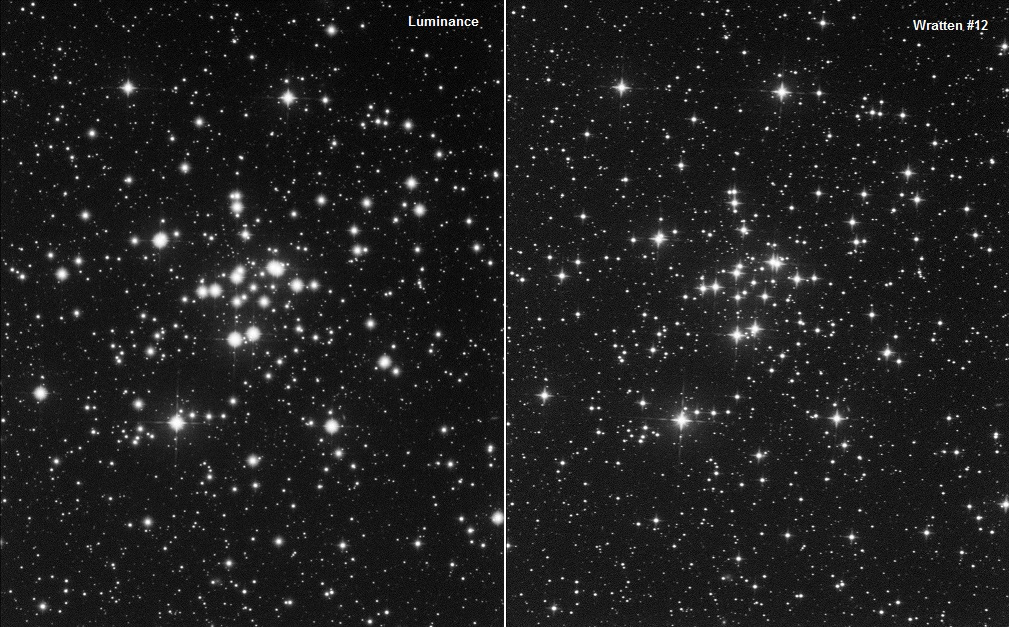
In my last post, I described how to capture tack-sharp images with my refractor by filtering out blue light using a Wratten #12 filter. The question remained: How can I capture color without blue?

The first thing to realize is that stars emit a continuum of colors from red to blue wavelengths. A red star strongly emits red light, but somewhat less blue. Likewise, a blue star strongly emits blue light, but somewhat less red. Green is sandwiched between red and blue. A red star is strong in red, less strong in green, and even less in blue. A blue star is strong in blue, less strong in green, and even less in red. We can take advantage of the difference between red and green to produce blue.

I borrowed a technique used in narrowband imaging. Narrowband filters are used for emission nebulae. Emission nebulae do not emit a continuum of colors. They emit discrete wavelengths. Most emission nebulae contain large amounts of hydrogen, varying amounts of oxygen, and some sulfur. The atoms are excited by the photons from nearby stars. Hydrogen emits several wavelengths but the prominent one is Hydrogen Alpha, abbreviated “Ha”. Ha emits light at the discrete wavelength of 6563 Angstroms. Doubly-ionized Oxygen, OIII, emits at 5007 Angstroms, and singly-ionized Sulfur, SII, emits at 6724 Angstroms. To the eye, SII is deep red, Ha is middle red, and OIII is bluish-green.

In narrowband image processing, it is common to assign SII to red, Ha to green, and OIII to blue. This is known as the SHO palette, made famous by the Hubble Space Telescope. SHO is also known as the Hubble Palette, but there are many other combinations that we can use. There is one called the HOO palette for cases where you only have Ha and OIII data. Exactly one year ago, I imaged the Tadpole Nebula in Ha and OIII. I used the HOO palette.

The HOO palette means that you assign Ha to red, and then split OIII, 50% to green, and 50% to blue. For my tastes, I am not fond of assigning 100% of Ha to red. It comes out screaming red which hurts my eyes. To soften it, I borrowed a technique from Sara Wager who splits Ha between red and green, and OIII between green and blue. The result is a pleasing reddish-orange for hydrogen and cyan for oxygen.

Now, getting back to the topic of this post. I only have data for the red and green filters, but I need to distribute it among red, green, and blue in order to make a color image. It sounds a lot like the HOO palette, doesn’t it? The solution is to split red filter data between the red and green channels, and to split the green filter data between the green and blue channels. It works remarkably well, although red stars appears slightly orange, and blue stars appear slightly cyan. All in all, I like the results. It gives me a way to breathe life into my refractor.

Technical details:

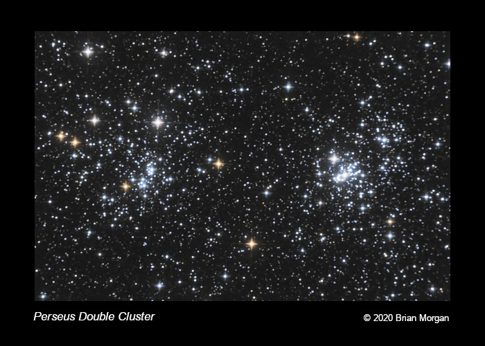
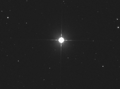
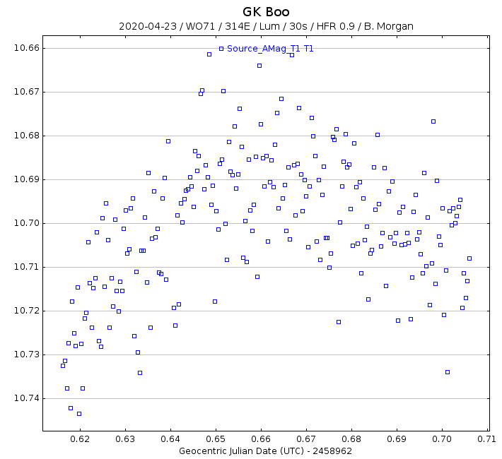
Perseus Double Cluster: NGC 869 and NGC 884

William Optics ZenithStar 71 Achromat
Atik 314E Mono CCD
GSO Wratten #12 filter as Luminance
Optolong Red and Green filters
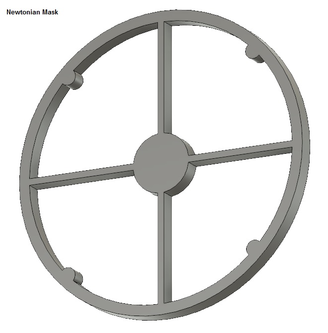
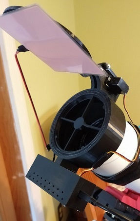
The Flatinator with Newtonian Mask

W12: 26x60s
R: 70x60s
G: 35x60s

Color Combine:
W12 => L
67% R => R
33% R + 33% G => G
67% G => B

Luminance filter vs Wratten #12

Luminance filter vs Wratten #12

Don’t be misled by deceptive marketing that promotes a refractor as “APO-like.” I fell for it because I am always looking for a good deal. Well, this deal didn’t pay off. In essence, I purchased an Achromat with ED glass. Frankly, I don’t know how much of an improvement the glass makes, but I recommend paying the price for an actual APO.

I have known for quite some time that my refractor cannot focus blue. Red is excellent, green is OK, but blue is a mess. Over two consecutive nights, I imaged M34. The left-hand image uses my standard Optolong luminance filter. The right-hand image uses a Wratten #12 (minus blue.) The comparison is stunning. Now all I need to do is figure out how to capture color!

Newtonian Mask

Newtonian Mask

I’ve only owned refractors. In my opinion, refractors are great for lunar and planetary imaging, but I have also seen outstanding images taken by fast refractors. Lately, I have become smitten by reflectors, although I do not own one. One thing I like is the diffraction pattern produced by the secondary mirror assembly. I wanted to see if I could simulate it using my refractor. I watched YouTube videos where people used dental floss stretched across the dew shield, but I wasn’t too happy with the results. So, I decided to create my own using a 3D printer.

The first attachment shows a 3D model of the profile of a secondary mirror and vanes, plus some imitation screws that add spice to the diffraction pattern. I created it using AutoDesk’s Fusion 360. The next attachment shows the mask inside my flat-field device, something I call “The Flatinator.” I built it two years ago from a concept I had. In the image, you can see the mask. It is held in there firmly by the surrounding structure, but there is still enough margin that I can rotate it to achieve any desired rotation angle.

I tested it two nights ago on the star, Almach, in Andromeda. It looks pretty spicy! Now I need to try it on a real target.

WASP-3 b Exoplanet Transit 2020-06-17

WASP-3 b Exoplanet Transit 2020-06-17

WASP-3 is a 10.7 magnitude star 3 degrees south of Vega in Lyra. WASP stands for Wide Angle Search for Planets. It consists of two robotic observatories in Spain and South Africa:

https://en.wikipedia.org/wiki/Wide_Angle_Search_for_Planets

Exoplanet “b” was discovered in 2007. It is a Jupiter-like planet 1.3 times the size of Jupiter. It revolves around WASP-3 every 1.846835 days. The duration of the transit is 137 minutes and its depth is 0.0123 magnitudes.

This is my second exoplanet, the first being HAT-P-5 b. Here is a write-up on it:

https://u235-varstar.now.sh/gallery/hat-p-5-b

You will notice that there is a lot of uncertainty in the data, nevertheless AstroImageJ was able to perform a transit model fit to my data.

Following that first experience I wanted to see what I could do to increase accuracy. Dr. Robin Glover suggested de-focusing as a technique to effectively turn my $400 camera into a $4000 camera.

Tonight I was not able to capture the entire transit from beginning to end but I did capture some high quality data for the second half. I de-focused as much as I could but there was a nearby 13th magnitude star only 18 arc-seconds away. Thankfully I set the exposure right, just below 55,000 ADU which is where my CCD begins to go non-linear.

Here are the results. I am very pleased with it:

WASP-3 b Exoplanet Transit

The next step would be to work out the relationship between three variables: Star magnitude, Magnitude error, and Aperture.

  • Aperture is equal to the amount of de-focus needed to achieve a certain star disc radius.
  • Magnitude error (the 3rd column in the spreadsheet) should be no greater than half the depth of transit, preferably smaller.

It should be possible to work this out mathematically but I think I will take the empirical approach to see how the data points cluster and then fit a curve to it.

The goal is to achieve consistent results instead of guessing. It’s OK to rely on experience but it would be great to have a heads-up in the planning stage to determine if a target is within the abilities of my equipment. For example, I can tell you that there is no way my kit could handle a 16th magnitude star with a transit depth of 0.005 magnitudes. It’s not going to happen but there are other scenarios where I can pull it off. Let’s say that the star is 8th magnitude then I know I can detect it just using the experience I’ve accumulated thus far. That’s fine but I want a more rigorous approach.

Eclipsing Binary Star System: V1053 Her

Eclipsing Binary Star System: V1053 Her

V1053 in Hercules is 13th magnitude that varies around 0.9 magnitudes from crest to trough. One of my goals was to determine a minimum exposure needed to produce satisfactory results. Satisfactory is subjective but for now I think that the “60-second data” is acceptable.

When I captured the image files I alternated between a 60-second exposure and a 30-second exposure for the entire 6.9-hour period. Due to my east-facing only imaging window I had to break it up into three sessions: May 14, 21, and 22. Afterwards I used AstroImageJ to calibrate and align the images, and then to perform differential photometry against a known constant-brightness star. If one were to look at the light curve taken by professionals you would see a noise-free sinusoidal pattern. Unfortunately the equipment required to reproduce such exceptional results are beyond my means. Instead I must settle for a certain degree of noise.

Notice that the 60-second plot (the top one) is less noisy than the 30-second plot (the bottom one). Furthermore, notice that there are outliers in the 30-second data, about an inch to the left of the red vertical “cursor”. This was part of the last session on May 22. The session started with the Sun only 16 degrees below the horizon, technically astronomical twilight, but true darkness arrived only 15 minutes later. The session lasted nearly 3 hours but notice how the outliers persisted for nearly half the session. My theory is that the atmosphere was “boiling” with turbulence. The interesting thing is this: notice how the outliers don’t exist in the 60-second data set. Here my theory is that doubling the exposure “averaged out” the negative effects of the turbulent atmosphere. I wonder if this has implications for conventional astrophotography? I’ll have to experiment with stacking two adjacent 30-second frames to see if it mitigates it.

One other interesting aspect to the light curve is that the “primary minimum” does not occur at exactly Phase: 0. I had a theory about this but then I researched it online and discovered that this is indicative of the existence of a large dark body that is perturbing the orbits of the stars: an Exoplanet!

Here is my new website that I developed for sharing my work with variable stars. The charts are fully interactive.

How to braid with four strands of wire

How to braid with four strands of wire

I am now onto my third stepper motor in two years. The motor is part of my self-designed right ascension drive system with periodic error correction.

When I designed the system I chose a specific stepper motor from an overseas manufacturer. I knew that one day the motor might need to be replaced so I purchased a half dozen. That first motor lasted more than a year but the second one for only a couple months. Such is the state of quality control. I am now onto my third one.

There are four wires coming out of the motor that can easily form a rat’s nest. You need to tame it or else sayounara. For the first motor I used “heat shrink tubing” seen here:

https://en.wikipedia.org/wiki/Heat-shrink_tubing

but I needed to chain quite a lot of them together to meet the requisite length of 20 inches. Furthermore I needed a “heat gun” in order to shrink the tubing. (If you are adventurous you can use a butane lighter.)

For the second motor I did not have enough tubing so I looked online for other solutions. I came across this 3-minute YouTube video on how to braid four strands (of anything):

It works for me although I should mention that you should ask your significant other to help straighten the wire before attempting to braid it. The stepper motor manufacturer did a poor job of preparing the wire for shipment. It looks like someone twirled it around their fingers a few times and then stuffed it in the box.

I’ve attached a photo of the braided wire after I got done. (Remember “Turn” and “Cross”, “Turn” and “Cross”…)

Eclipsing Binary Star System: GK Boo (Part 2)

Eclipsing Binary Star System: GK Boo (Part 2)

The data that I presented in Part 1 was from a single session on April 23, 2020 however I also captured data on April 19, 2020 but unfortunately it suffered from poor tracking. Nevertheless it is still useful for demonstration purposes.

Before I present the second data set allow me to briefly describe the software I use:

AstroImageJ, henceforth referred to as AIJ, enables me to calibrate and align frames (and stack if I so wish.) More importantly I can perform Differential Photometry. The one drawback from my perspective is that it is designed for Exoplanet research and therefore expects me to capture the entire light curve in a single session, however my requirements differ in that the period of most variable stars far exceeds that.

VStar, a Java application from AAVSO, enables me to view my data over multiple sessions. Using it I can switch between two modes: Light Curve and Phase Plot. Light Curve mode is similar to AIJ in which the horizontal axis is in units of time. Phase Plot mode requires me to know something about the period of the light curve. It takes that information and then “folds” my observations onto a phase scale from -100% to +100%.

In the following screenshot I used VStar to plot the two sessions in Light Curve mode. Notice how the data is compressed horizontally. This is due to the fact that four days separated the first and second session:

Above: VStar plot of two sessions in Light Curve mode.

This next screenshot uses VStar’s Phase Plot mode. I entered GK Boo’s period obtained from the AAVSO database:

Above: VStar plot of two sessions in Phase Plot mode.

Compare the Phase Plot of my data to that of all data from members of AAVSO, seen below. (Please ignore the red box drawn atop one of the peaks. This image is being shared from an earlier post.) Notice the similarity:

VStar Phase Plot of GK Boo from all data available in the AAVSO database.

Phase Plot mode is essential since some variable stars take a year or more to capture and can span dozens of sessions.

Recreating Edwin Hubble’s discovery of a Variable Star in the Andromeda Galaxy

Recreating Edwin Hubble’s discovery of a Variable Star in the Andromeda Galaxy

On October 6, 1923 renowned astronomer Edwin Hubble discovered a pulsating star in the Andromeda Galaxy which quickly led to the revolutionary discovery that M31 is a galaxy unto itself 2.5 million light-years away, and not a gaseous cloud of stars within our own Milky Way.

I dipped into my archive of astro images to see if I might have captured that same variable star. I did! In the attached image I’ve overlaid a small region of a 6-panel mosaic I made last year, atop Hubble’s photographic plate he captured with the 100-inch telescope at Mount Wilson Observatory. You can see that the pattern of stars matches nicely. At the point of the arrow that I marked “VAR!” you will see an equilateral triangle of faint stars. You can see that it matches up with Hubble’s. That one star at the vertex of the triangle is the famous variable star.

My image is a stack of 21x 90-second luminance frames captured with a cooled Atik 314E CCD and William Optics 71mm f/5.9 refractor under Bortle 5 skies. Total integration time is 31.5 minutes. I know nothing of the period of this variable star. Being a Cepheid type variable star its period is most likely one or more days in length, so integrating for 31.5 minutes is not a problem. The bigger question is, am I seeing it at minimum light or maximum light? I almost don’t want to know. I want to feel the same sense of discovery as Hubble did.

EDIT: I suspect that this variable star is likely to have a long period perhaps months long. I suspect this because of the “period-luminosity relationship” which says that highly luminous Cepheids have long periods. This star must be highly luminous if I can see it as a point source from such a great distance. If it was less luminous it would be lost in the glow of the galactic arms.

I will make this one of my top priority projects this Fall: measure the period of the variable star, and then calculate its distance using Leavitt’s Law.

https://apod.nasa.gov/apod/ap200426.html
https://apod.nasa.gov/apod/ap950701.html
https://astrotuna.com/andromeda-galaxy-mosaic-as-of-2019-08-12/

AAVSO’s official designation is M31 V0619. They report that its magnitude fluctuates between 18.5 and 19.8V. That is faint. I’ve known that my scope/cam can see down to 18th magnitude at my Bortle 5 site but can it see down to 19th magnitude? What makes things worse is that the star is embedded in the glow of a spiral arm which further reduces the signal-to-noise ratio. There is only one way to tell. Do it!

I was curious as to what phase the star was in when I captured my image. According to the AAVSO’s Ephemeris it reached maximum light on July 31, 2019 07:08 UTC. My image was captured August 3, 2019 02:00 UTC. So, three days after maximum light. That pretty much puts it at magnitude 18.5.

Here is the Phase Plot contributed by ten AAVSO members between 2010 and 2019. Ignore the outliers.

VStar Phase Plot of Edwin Hubble’s revolutionary Cepheid variable star.
100th Anniversary of Astronomy’s Great Debate

100th Anniversary of Astronomy’s Great Debate

Today’s NASA Astronomy Picture of the Day (APOD) is a celebration of the 100th anniversary of astronomy’s Great Debate held at New York’s Museum of Natural History between Harlow Shapley and Heber Curtis. Shapley argued that the Milky Way was the size of the known universe and that the Andromeda Nebula (M31) was part of it just like the Orion Nebula (M42). The debate ended with no decision either way. In fact Shapley’s model was accepted for years until Edwin Hubble and Henrietta Leavitt revolutionized the scale of the universe and proved that the Andromeda Nebula was in fact its own independent galaxy. 100 years ago today!

https://apod.nasa.gov/apod/ap200426.html
https://en.wikipedia.org/wiki/Great_Debate_(astronomy)
https://en.wikipedia.org/wiki/Edwin_Hubble
https://en.wikipedia.org/wiki/Henrietta_Swan_Leavitt
https://en.wikipedia.org/wiki/Harlow_Shapley
https://en.wikipedia.org/wiki/Heber_Doust_Curtis

What makes this anniversary relevant to the topic of Variable Stars is that it was Hubble’s discovery of a Cepheid type variable star in the Andromeda Galaxy. Coincident with this discovery, his associate Henrietta Leavitt had painstakingly measured Cepheid variables in the Milky Way and discovered Leavitt’s Law which relates the distance of a star with its period and apparent magnitude. With this knowledge Hubble and Leavitt proved Shapley’s model was incorrect.

Many of us associate the famed Hubble Space Telescope with spectacular visual images of the deep sky but in reality it is equipped with state-of-the-art photometers that continue the pioneering work of Edwin Hubble and Henrietta Leavitt. As a result Leavitt’s Law was modified to include adjustments for the effects of interstellar dust.

Eclipsing Binary Star System: GK Boo (Part 1)

Eclipsing Binary Star System: GK Boo (Part 1)

Photometry with your CMOS or CCD camera has always been and continues to be of great importance to science. There are many different types of variable stars. There are Cepheid type stars that are useful for measuring the distance to galaxies, and then there are Eclipsing types of which ‘GK Boo’ is one.

The ‘GK Boo’ binary system consists of two spectral class M stars (red) that revolve around a common center of mass every 11 hours 28 minutes. You can set your watch by it. When you think about it, it is incredible when you consider that Jupiter rotates around its polar axis every 9 hours 55 minutes yet these two massive stars revolve around each other every 11.5 hours! Think about what that must look like from a hypothetical planet. It’s the stuff of Science Fiction.

The entire light curve of ‘GK Boo’ cannot be captured in a single night so it must be spread out over multiple sessions. I will be using two software applications to make this work: AstroImageJ and VStar. I’ll have more to say about these in Part 2 of this series.

Anyhow here is the result of last night’s work:

This is a plot of 240x 30-second frames that spanned 2 hours time. Each frame was calibrated and aligned using AstroImageJ. To measure the small light fluctuations I compared the pixel values of the variable star to the pixel values of a nearby constant-brightness star.

Light Curve of ‘GK Boo’ spanning 2 hours on 2020-04-23 (AstroImageJ)

And here is a plot of the entire light curve of ‘GK Boo’ over its entire period. The data came from AAVSO’s database. I’ve drawn a rectangle around the 2 hour time span that I captured. Notice the similarity of shape.

Over the course of the next several days, weather permitting, I will capture more data that will fill in the rest of the period.